March 13, 2024
Summary: in this tutorial, you will understand cost estimation for sequential scan.
Table of Contents
PostgreSQL Sequential Scan
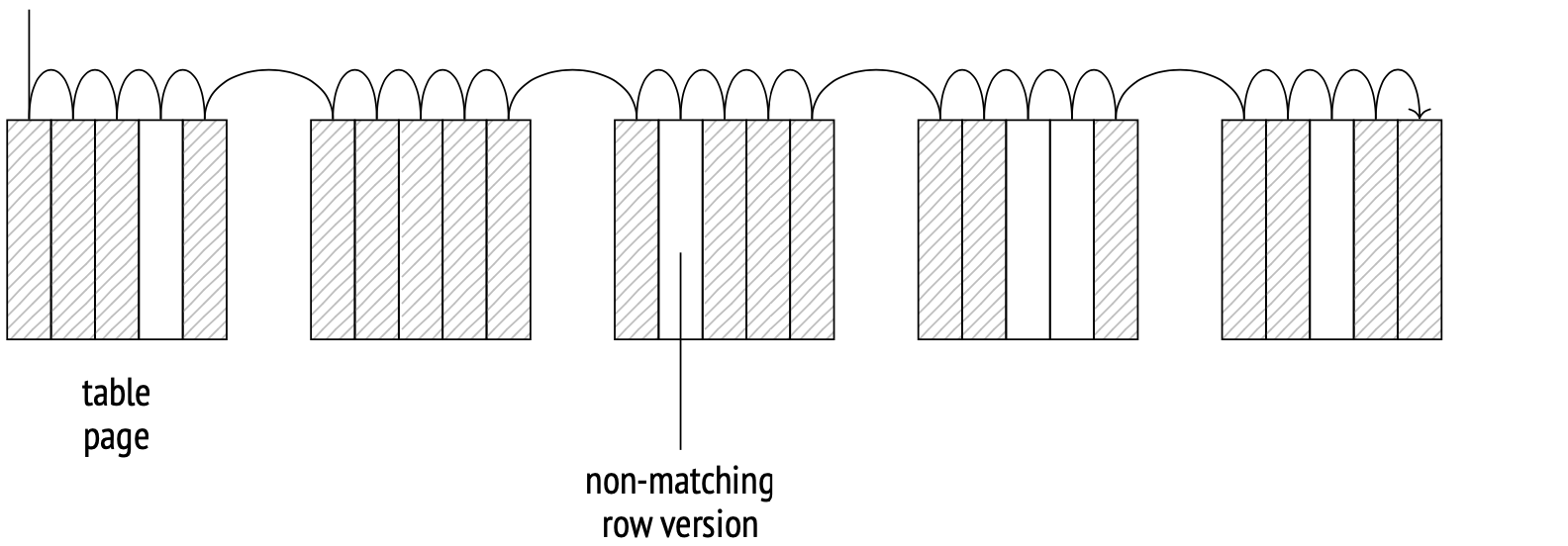
The storage engine determines how table data is physically distributed on disk and provides a method to access it. Sequential scan is a method that scans the file (files) of the main table fork entirely. On each page, the system checks the visibility of each row version, and also discards the versions that don’t match the query.

The scanning is done through the buffer cache. The system uses a small buffer ring to prevent larger tables from pushing potentially useful data from the cache. When another process needs to scan the same table, it joins the buffer ring, saving disk read times. Therefore, scanning does not necessarily start from the beginning of the file.
Sequential scan is the most cost-effective way of scanning a whole table or a significant portion of it. In other words, sequential scan is efficient when selectivity is low. At higher selectivity, when only a small fraction of rows in a table meets the filter requirements, it’s usually better to use index scan.
Example plan
Let’s start with a little test setup:
CREATE TABLE test7 (id integer, status integer, str text);

INSERT INTO test7 (id, status, str)
  SELECT i, CAST(random() * 15 AS int), 'xxx'
    FROM generate_series(1, 200000) AS s(i);

ANALYZE test7;
A sequential scan stage in an execution plan is represented with a Seq Scan node.
EXPLAIN SELECT * FROM test7;

                          QUERY PLAN
--------------------------------------------------------------
 Seq Scan on test7  (cost=0.00..2695.00 rows=200000 width=12)
(1 row)
Row count estimate is a basic statistic:
SELECT reltuples FROM pg_class WHERE relname = 'test7';

 reltuples
-----------
    200000
(1 row)
When estimating costs, the optimizer takes into account disk input/output and CPU processing costs.
The I/O cost is estimated as a single page fetch cost multiplied by the number of pages in a table, provided that the pages are fetched sequentially. When the buffer manager requests a page from the operating system, the system actually reads a larger chunk of data from disk, so the next several pages will probably be in the operating system’s cache already. This makes the sequential fetch cost (which the planner weights at seq_page_cost, 1 by default) considerably lower than the random access fetch cost (which is weighted at random_page_cost, 4 by default).
The default weights are appropriate for HDD drives. If you are using SSDs, the random_page_cost can be set significantly lower (seq_page_cost is usually left at 1 as the reference value). The costs depend on hardware, so they are usually set at the tablespace level (ALTER TABLESPACE ... SET).
SELECT relpages, current_setting('seq_page_cost') AS seq_page_cost,
  relpages * current_setting('seq_page_cost')::real AS total
FROM pg_class WHERE relname='test7';

 relpages | seq_page_cost | total
----------+---------------+-------
      695 | 1             |   695
(1 row)
This formula perfectly illustrates the result of table bloating due to late vacuuming. The larger the main table fork, the more pages there are to fetch, regardless of whether the data in these pages is up-to-date or not.
The CPU processing cost is estimated as the sum of processing costs for each row version (weighted by the planner at cpu_tuple_cost, 0.01 by default):
SELECT reltuples,
  current_setting('cpu_tuple_cost') AS cpu_tuple_cost,
  reltuples * current_setting('cpu_tuple_cost')::real AS total
FROM pg_class WHERE relname='test7';

 reltuples | cpu_tuple_cost | total
-----------+----------------+-------
    200000 | 0.01           |  2000
(1 row)
The sum of the two costs is the total plan cost. The plan’s startup cost is zero because sequential scan does not require any preparation steps.
Any table filters will be listed in the plan below the Seq Scan node. The row count estimate will take into account the selectivity of filters, and the cost estimate will include their processing costs. The EXPLAIN ANALYZE command displays both the actual number of scanned rows and the number of rows removed by the filters:
EXPLAIN (analyze, timing off, summary off)
SELECT * FROM test7 WHERE status = 7;

                                       QUERY PLAN
-----------------------------------------------------------------------------------------
 Seq Scan on test7  (cost=0.00..3195.00 rows=13060 width=12) (actual rows=13474 loops=1)
   Filter: (status = 7)
   Rows Removed by Filter: 186526
(3 rows)
Example plan with aggregation
Consider this execution plan that involves aggregation:
EXPLAIN SELECT count(*) FROM test7;

                            QUERY PLAN
-------------------------------------------------------------------
 Aggregate  (cost=3195.00..3195.01 rows=1 width=8)
   ->  Seq Scan on test7  (cost=0.00..2695.00 rows=200000 width=0)
(2 rows)
There are two nodes in this plan: Aggregate and Seq Scan. Seq Scan scans the table and passes the data up to Aggregate, while Aggregate counts the rows on an ongoing basis.
Notice that the Aggregate node has a startup cost: the cost of aggregation itself, which needs all the rows from the child node to compute. The estimate is calculated based on the number of input rows multiplied by the cost of an arbitrary operation (cpu_operator_cost, 0.0025 by default):
SELECT
  reltuples,
  current_setting('cpu_operator_cost') AS cpu_operator_cost,
  round((
    reltuples * current_setting('cpu_operator_cost')::real
  )::numeric, 2) AS cpu_cost
FROM pg_class WHERE relname='test7';

 reltuples | cpu_operator_cost | cpu_cost
-----------+-------------------+----------
    200000 | 0.0025            |   500.00
(1 row)
The estimate is then added to the Seq Scan node’s total cost.
The Aggregate’s total cost is then increased by cpu_tuple_cost, which is the processing cost of the resulting output row:
WITH t(cpu_cost) AS (
  SELECT round((
    reltuples * current_setting('cpu_operator_cost')::real
  )::numeric, 2)
  FROM pg_class WHERE relname = 'test7'
)
SELECT 2695.00 + t.cpu_cost AS startup_cost,
  round((
    2695.00 + t.cpu_cost +
    1 * current_setting('cpu_tuple_cost')::real
  )::numeric, 2) AS total_cost
FROM t;

 startup_cost | total_cost
--------------+------------
      3195.00 |    3195.01
(1 row)

